Goodwill Valuation for Impairment Testing During Recession

By CHUA KIM CHIU and HO YEW KEE
PITFALLS AND CHALLENGES
For companies with business acquisitions, goodwill forms a substantial percentage of their total assets and equity. For example, as at 31 March 2020, Singtel has more than $11 billion goodwill balance on its balance sheet, constituting about 25% and 40% of its total assets and equity, respectively. Goodwill is also usually a material item discussed in audit reports under key audit matters.
In this time of unprecedented economic uncertainty, businesses and cash flows have been disrupted. For the first half of 2020, companies should take a hard look at the carrying amount of goodwill and ask whether its recoverable amount (RA) might have fallen below the carrying amount. This is becoming more probable when asset values have declined generally due to the current economic recession.
This article will first provide a brief overview of the accounting for goodwill impairment and then discuss certain pitfalls and challenges in goodwill valuation for impairment testing in the context of the current recession.
IMPAIRMENT AND RECOVERABLE AMOUNT OF GOODWILL
Accounting for goodwill is covered by three financial reporting standards: Singapore Financial Reporting Standard (International) (SFRS(I)) 3 Business Combinations, SFRS(I) 1-36 Impairment of Assets and SFRS(I) 1-38 Intangible Assets.
The acquirer of a business must allocate the acquisition price to the acquiree’s identifiable tangible and intangible assets, liabilities and contingent liabilities at their fair values at the date of acquisition and the remaining balance to goodwill1.
An entity must test goodwill for impairment at least annually and whenever there is an indication of impairment2. Goodwill is impaired whenever its RA falls below the carrying amount3. There is no requirement to assess whether the shortfall is temporary or permanent. Also, goodwill impairment charge cannot be reversed subsequently4. Therefore, we may intuitively view the impairment-only approach as an ad hoc allocation of the cost of goodwill to the income statement.
RA is the higher of the asset’s fair value less costs of disposal (FVLCOD) and its value in use (VIU)5. Costs of disposal refer to transaction costs such as advertising or broker’s commission6. Here, an asset can be either an individual asset item or a business unit known as a “cash generating unit” (CGU)7.
Fair value of an asset is the price that would be received to sell the asset in an orderly transaction between market participants at a point in time, with reference to assumptions a hypothetical market participant would use in valuing the asset8.
VIU is a valuation from the current owner’s perspective, based on benefits the owner is capable of generating through its specific use of the assets9. VIU may differ from FVLCOD, when the specific use by the owner may be unique.
To summarise:
Impairment loss = Carrying amount – Higher (FVLCOD, VIU)
VALUING THE CGU THAT CARRIES THE GOODWILL
Upon acquisition, the acquirer must identify and allocate the total acquired goodwill to the acquirer’s various CGUs at the lowest possible level10. This is to facilitate subsequent goodwill impairment testing at the CGU level.
Goodwill does not generate cash flows independently of the other assets in the CGU. Instead, it is an economic resource capable of generating future economic benefits in combination with other assets in the CGU that carries the goodwill11. Hence to test goodwill for impairment, one must value the CGU12.
PRACTICAL APPLICATION OF THE DCF VALUATION MODEL
We surveyed the latest financial statements of the 10 largest companies, based on market capitalisation, listed on the Singapore Exchange (SGX) and noted that they used the Discounted Cash Flow (DCF) models to estimate the VIU of the CGU for goodwill impairment testing.
It is a common practice to divide the future cash generating time horizon of a CGU into two phases:
- Phase 1: The CGU usually uses its best estimates of the expected cash flows for the next five years based on budgets, forecasts and projections.
- Phase 2: The CGU usually uses the cash flow for Year 5 (base-year cash flow) to project the cash flows for the remaining years to perpetuity using an estimated growth rate, denoted by g. The present value at the end of Year 5 representing all subsequent future cash flows beyond Year 5 is called the terminal value (TV). This TV needs to be further discounted to become a present value at the valuation date (PVTV).
To summarise, VIU is the sum of two components:
- The present value of the projected cash flows in Phase 1 (PV-Phase 1), and
- The present value of the projected cash flows in Phase 2 (PVTV).
Given its shorter duration compared to the remaining life of a going concern or a long-term project, PV-Phase 1 would normally make up less than 50% of the total value of a VIU13. Therefore, PVTV, being highly sensitive to the inputs to the model, that is, the base-year cash flow, the risk-adjusted required rate of return or discount rate (k) and the estimated earnings growth rate (g), can significantly affect the VIU of a CGU.
PITFALLS AND CHALLENGES
We will highlight two major pitfalls and challenges in real-life valuation, especially in times of recession. Our intention is to help companies avoid these pitfalls through a better understanding of the assumptions, concepts and application of the DCF model.
Pitfall 1: Mis-estimation of discount rate
The current depressed stock prices reflect the combined effect of lower future cash flows and higher discount rates assumed by market participants due to poorer business prospects and heightened investment risk.
The discount rate is a crucial input to the valuation of a CGU. The 10 largest SGX companies which we surveyed disclosed pre-tax discount rates for recent goodwill valuations to be ranging from 5% to 16%. The actual discount rates used in valuation are lower when expressed on a post-tax basis.
The valuation practitioners tend to rely on the one-factor capital asset pricing model (CAPM) to estimate the discount rate for a CGU. CAPM is often misunderstood as a magic formula into which one can input the historical values to obtain an estimate of the current discount rate. This is fallacious. Whenever we input a historical parameter into the CAPM, we are making an implicit assumption that the historical pattern continues to prevail today. This is difficult to justify when the economy has changed so drastically in the last few months.
Based on our recent observations, we have increasingly seen companies combining current with historical data to derive the discount rate for the CGU. For example, they have been quick to use the current low government bond yield as the proxy for risk-free rate (Rf) together with the same historical market risk premium (Rm – Rf) of about 5% to 6% and the same historical beta (β) for the CGU, as inputs into the CAPM below to derive the discount rate, k, for the CGU:
k = Rf + β (Rm – Rf)
As a result, the estimated k is lower than before. Despite deteriorating projected future cash flows, this lower k will result in a sustained VIU and in turn, RA of the CGU. However, this outcome is counterintuitive in a recession and is not in line with a higher market risk premium implied in depressed stock prices. Based on simulated sensitivity analysis, if the unbiased estimate of k is 10%, ceteris paribus, a one percentage point estimation error in k would change PVTV by about 13%. The use of low discount rates for CGU and goodwill valuation is not uncommon in practice and the Covid-19-induced economic recession has amplified this issue.
Pitfall 2: Mis-estimation of free cash flows
When estimating free cash flows in the DCF model, a capital expenditure is a cash spending that effectively reduces the valuation and the subsequent depreciation is a cash saving (non-cash expense) that effectively increases the valuation. Under the DCF model, valuation is driven by free cash flows and adjustments must be made to convert the “accrual accounting net profit” (AANP) to an adjusted “cash accounting net profit” (CANP).
Table 1 illustrates this concept with an assumed discount rate of 10% in three scenarios, A, B and C. Row 1 is the AANP for the next five years. Row 2 shows the planned capital expenditure and depreciation. Row 3 is the CANP.
In Scenario A, across the five years, a cash capital expenditure is deducted upfront and all the annual depreciations are added back in subsequent years. The total adjustments will self-balance to zero on an undiscounted basis.
Assuming the present value of 739 (A3) to be a more accurate valuation and 758 (A1) is an approximation, the estimation error of 19 is less than 3%, which is hardly material when valuation is inherently a broad estimate. This is in contrast to a big swing in valuation from a small change in one of the inputs like the discount rate or the growth rate. This is also much smaller than the potential distortions from the pitfalls illustrated below.
A common pitfall found in practice is that not all the offsetting cash flow adjustments are captured within the five-year period. This would be the case if the capital expenditure had occurred just before Year 1 (Scenario B) or is projected to occur in Year 4 (Scenario C).
B2 shows how missing a capital expenditure adjustment can artificially increase the valuation by about 13% from 739 to 837 (B3).
C2 shows how missing three depreciation adjustments can artificially decrease the valuation by about 5% from 739 to 705 (C3).
Table 1 Cash accounting net profit adjustments
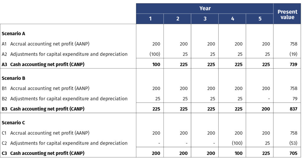
This “cash flow adjustment imbalance” is another common pitfall seen in practice. Often, this valuation distortion is not detected as it is obscured by the combined effects of other valuation inputs.
An extension of the above pitfall is the use of a base-year cash flow to project future free cash flows to infinity. For example, if the base-year AANP, depreciation and CANP resemble that of Year 2 under Scenario A, the positive cash flow effect of the base-year depreciation will be repeated as an annual free cash flow (cash saving), growing exponentially to infinity without any capital expenditure (cash spending). This is a “free cash ever after fallacy” that will inflate the valuation. It is fairly common in practice probably because some textbook examples have unwittingly illustrated this approach.
We have personally observed companies using a current CANP that is materally higher than AANP, with one that is 20% to 30% higher due to a low net profit base coupled with a high annual depreciation/amortisation. The end result is a grossly inflated valuation.
This pitfall can be potentially avoided by using AANP for the year as a proxy for CANP. This is on the condition that the AANP is not affected by significant unusual or exceptional items for the year. Net profits would be a close approximation to free cash flows for the year if it is a group’s practice to replace depreciated assets progressively and evenly over time instead of intermittently. In practice, for modelling annual cash flows, it is not uncommon for practitioners to smooth out the erratic pattern on the assumption that the annual depreciation is contemporaneously replaced by capital expenditure. This helps to avoid the pitfall.
The key lesson here is that the base-year cash flow measure for projecting into the future must be a good representation of the CGU’s expected future cash flows.
The Covid-19 situation has compounded the free cash flow estimation problem. The pace of recovery is highly uncertain. Projecting future cash flows in times of great uncertainty is highly subjective and prone to being overly optimistic or pessimistic. In times like this, the corporate governance structure around the valuation process, including review by the audit committee, independent directors and external auditors will become even more critical in providing the needed checks and balances to make objective and reliable accounting estimates. Governing authorities need to know it is not business as usual this time for goodwill impairment and they need to have assurance that the assessment is properly carried out.
CONCLUDING REMARKS
The Covid-19 pandemic and the ensuing recession pose a significant challenge to accounting for goodwill impairment. For the coming half-yearly reporting season, companies will need to conduct their goodwill impairment testing with more rigour as the likelihood of impairment has risen significantly. It is important to apply a good understanding of the assumptions, valuation concept and good business sense beyond number crunching. This article provides a quick rendition of some of the major pitfalls to avoid. Given the assumptions and judgements around the use of the DCF model, good corporate governance will provide the much-needed checks and balances.
Chua Kim Chiu is Professor (Practice) of Accounting, NUS Business School, National University of Singapore. Ho Yew Kee is Professor and Associate Provost, Singapore Institute of Technology.
1 SFRS(I) 3, paras 18 and 32
2 SFRS(I) 1-36, para 90
3 SFRS(I) 1-36, paras 6 and 8
4 SFRS(I) 1-36, para 124
5 SFRS(I) 1-36, paras 6, 18 and 74
6 SFRS(I) 1-36, para 28
7 SFRS(I) 1-36, para 18
8 SFRS(I) 1-36, para 6
9 SFRS(I) 1-36, para 30
10 SFRS(I) 1-36, para 80
11 SFRS(I) 1-36, para 81
12 SFRS(I) 1-36, para 90
13 There could be exceptions for short-term projects or businesses that generate exceptionally high cash flows for a few initial years.
This article was first published in the ISCA Journal. You can read the original version here.


